Although the idea of vehicle detection is not a groundbreaking one and has been around since the emergence of video cameras and embedded sensors, these methods were often marred by high capital and maintenance costs and a high complexity from having to integrate multiple data sources, each with a limited band of inputs. The prevalence of drones in the commercial market in recent years on the other hand, has brought about a new era of state-of-the-art aerial photogrammetry and a drastic reduction in the cost of obtaining aerial data. With this sudden increase in information, and by combining machine learning with GIS technologies, we are now capable of performing new and insightful analyses on issues of interest.
Existent business problems which stand to benefit from this include customer flow analyses and demographic modelling. This is particularly useful for those in the retail sector looking to monitor peak business hours by counting the number of parked vehicles at a given time and also extrapolate useful customer information (such as income, marital status, household size and even political inclination) by classifying the types of vehicles they own.
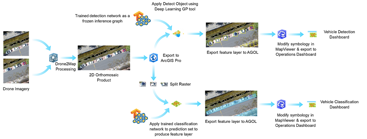
So, can we solve these problems using AI and GIS? The answer is yes, and a good starting point would be to come up with a workflow that tallies the number of cars per unit time as well as infer the vehicle type for every positive detection. In this article, I aim to give a comprehensive overview of a such a workflow — from data acquisition and processing using Drone2Map to performing data inferencing using TensorFlow and ArcGIS Pro, and finally to creating actionable BI visualizations using The Operations Dashboard in ArcGIS Online (AGOL).
Data Collection & Exploratory Analysis using Drone2Map
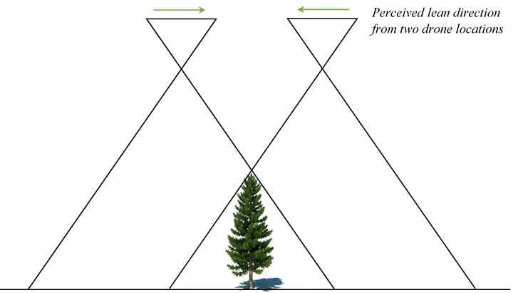
To obtain some sample data, we flew a drone over a busy parking lot here at our office in Redlands, California and obtained a series of geo-tagged tiff files with geolocation corroborated by 5 ground control points (GCPs) to ensure the result would be accurate enough to identify the correct parking space for each vehicle. These images were captured along a “lawn mower” flight path with an overlap of 70% along flight lines and at least 60% between flight lines. The reason we do this is to facilitate the generation of true orthomosaics. Traditional orthos (or “frame” orthos) suffer from what is known as the “layover effect”, where tall structures such as trees or buildings seemingly “lean” toward or away from the observer as a consequence of stitching together disparate frames that do not capture objects at a true nadir perspective. This effect worsens for objects that are at the edges of a drone’s field of view.
Using Drone2Map, we can take these individual frames and resolve for an object’s true ortho by finding common views between a frame and its 8 adjacent frames in a point cloud and then keeping the views that have a high degree of overlap. The resultant orthomosaic is not only a true ortho, but one that does not reveal seamlines between images typical of frame orthos.
Of course, all of this is automated, and the actual image processing step is simple: Create a 2D mapping project in Drone2Map, pull in your data, add ground control points as needed and then hit start to generate a true orthomosaic.
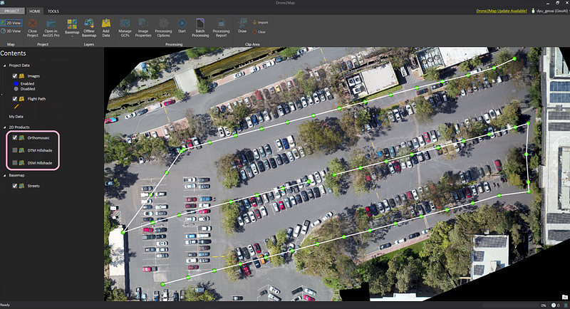
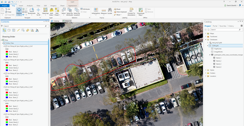
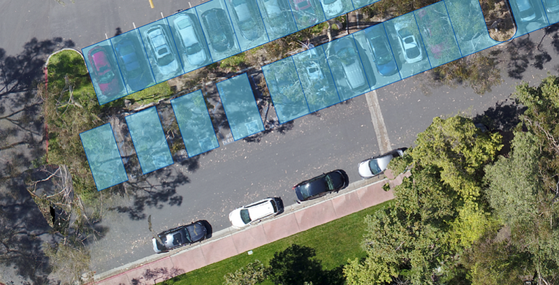
From this, we obtain 3 classes of output products: A 2D orthomosaic of our parking lot, a digital surface model (DSM) layer and a digital terrain model (DTM) layer. An initial thought was to simply pass the DSM to a detection network to produce bounding boxes on distinctly “car-like” protrusions. However, on closer inspection of the dataset we identified some potential issues with this approach: in this particular parking lot, the coverage of foliage was so extensive as to affect the detection of certain cars partially or completely hidden by overhanging branches and leaves.
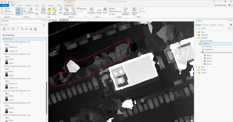
The overhanging vegetation affected both the DSM and orthomosaic, but since the edge of each image includes oblique view angles at the image edges, some images were able to view partially or completely underneath the tree canopy. ArcGIS also enables each image from the drone to be orthorectified. Following photogrammetric processing in Drone2Map, each image could be analyzed in its proper geospatial placement, providing multiples views of each parking space.
Processing of these oblique views was beyond the scope of this initial project, but will be the subject of future testing. In addition, parts of the canopy depicted by the orthomosaic are not fully opaque, and the RGB bands may also provide additional channels that would allow correct subdivision of vehicles into categories such as trucks, sedans and SUVs. From a data collection standpoint, it is also much easier to collect pure ortho imagery than outfitting drones with LIDAR sensors for DSM/DTM detection.
Simple Approach: Building a classification model using InceptionV3
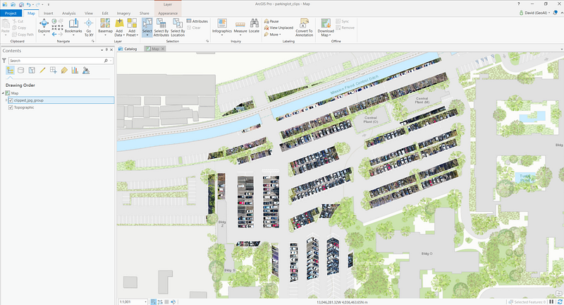
Our first solution for tackling this problem was an obvious one: Simply overlay a polygon layer from a mapped parking lot on top of the orthomosaic raster and clip out cars using the Split Raster geoprocessing tool to get our prediction set. This was very easily done.
Then comes the question of which classification model to apply atop which finetuning set. A simple off-the-shelf model that’s available from both TensorFlow Slim and TensorFlow Hub is InceptionV3. Based off the original InceptionNet (Szegedy et al.), this third revision bears much resemblance in terms of core structure to the original with similar component modules. However, it has the addition of factorization methods to reduce the representational bottleneck as well as label smoothing and batch norm operations on the auxiliary classifiers to increase regularization.
As with most TensorFlow Hub models, there is no need to train from scratch when we can apply transfer learning; Luckily, InceptionV3 was pretrained on ImageNet.
As for the finetuning set, The Cars Overhead with Context (COWC) dataset from LLNL was an easy pick for its richly annotated set of 32,716 vehicles as well as hard negative examples (boats, commercial vehicles etc.). Although the dataset doesn’t plug straight into the classification network, the only preprocessing work here involves reading through the list of the annotated text files and cropping the associated jpegs with either OpenCV or ImageMagick. (N.B. the COWC dataset has 4 class labels: Sedan, Pickup, Others and Unknown. With an additional background class that makes 5 classes. I had to play around with class balancing to ensure each class was sufficiently represented, and also mine some samples for background classes which weren’t provided in COWC).
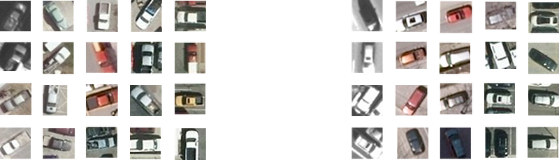
These images have been extracted from the original COWC format which is comprised of large 22000x22000 images with bounding box information contained in ancillary .txt files. One thing to note is that the original bounding box coordinates tended to crop off large sections of the vehicles in question, which ultimately lead to worse overall performance in identifying the pickup class. Therefore these images have all been cropped using larger 34x34 bounding boxes.
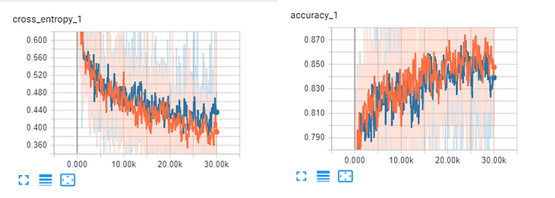
By looking at the COWC dataset we can immediately tell that the resolution of the dataset is not ideal. Early training results have shown that the classification network performed exceedingly well in binary classification tasks of identifying occupied/unoccupied spaces, but performed worse in distinguishing between vehicle classes. Part of the reason for this is also due to the fact that the pickup class was severely underrepresented. Testing proved that undersampling the sedan/other/background classes yielded the best validation accuracy (as opposed to oversampling the pickup class).
Once the model was sufficiently trained (on a good GPU this takes a couple hours — for me it was a Tesla K80 on the GeoAI VM for about 1.5 hours at a training accuracy of 0.85 and a validation accuracy of 0.84), we can proceed to apply our previously extracted prediction set to the model.
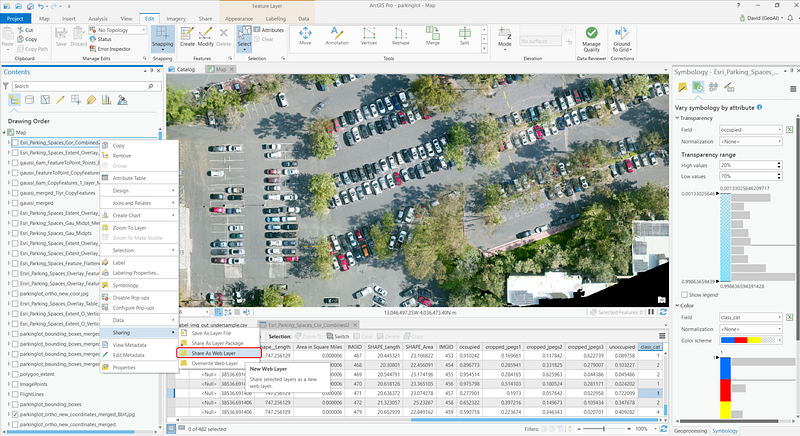
Output these results into a .csv file (it might be useful to apply some smart naming conventions here to ensure your data items match the OBJECTIDs of each polygon in the parking space feature layer. From here, simply combine the two layers using Add Join and voilà, you have a polygon layer that associates a class probability with each parking space based on an aerial image you took.
Thus far, we have only created some rich geotagged layers that are not yet informative nor intuitive enough give any kind of analytical insight. This is where ArcGIS Online offers us a path forward: we export both the orthomosaic as well as the feature layer to our ArcGIS Online Portal, then optionally in the MapViewer, modify the symbology of our polygon layer to be attribute-driven.
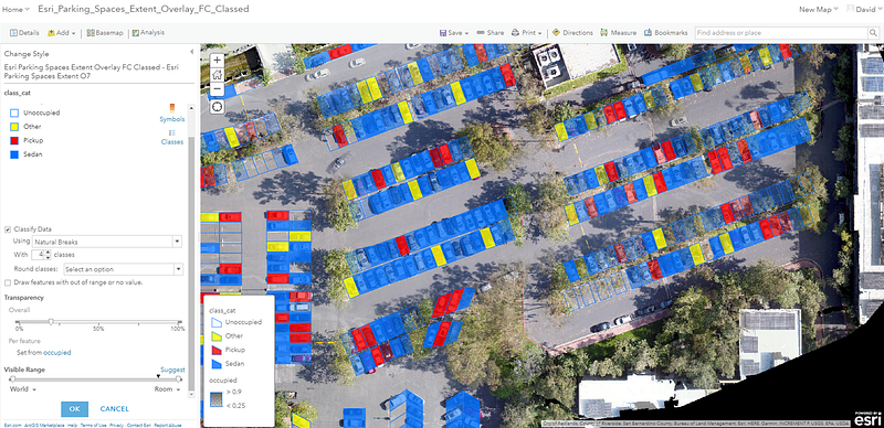
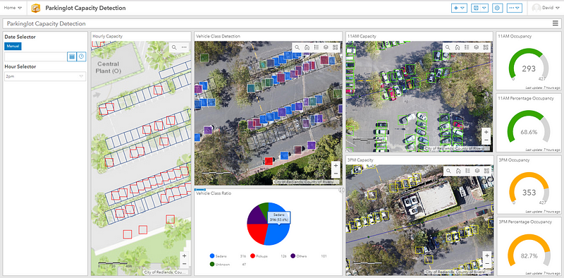
You can then import individual maps and visualize the results interactively on the Operations Dashboard:
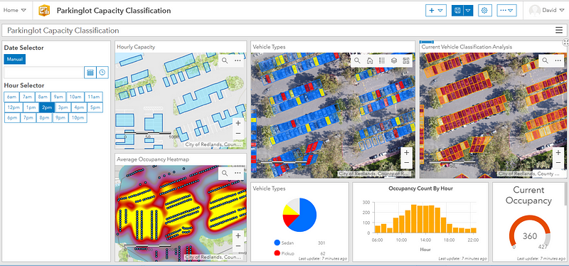
We scheduled two drone flights over the same parking lot at different times of the day. To complement this data, we have also generated some mock input to illustrate occupancy info on an hourly basis that simulates customer flow within a typical work day. The Hour Selector cycles through parking patterns over every time segment. To suit your use case, you may also decide to deploy a drone every few weeks or every few months. The Average Occupancy Heatmap is a visual representation of “hot spots” wherein vehicles aggregate. If you like it is also possible to generate a “Turnover Heatmap” that maps regions in which vehicles are likely to park for longer/shorter periods. Both of these views are potentially useful for understanding demographic behavior when crossed-referenced with vehicle types or to detect favorite stores & customer stay-times at shopping venues.
The two useful vehicle categories from COWC: sedans and pickups, are shown in the Vehicle Types visual element, each color coded and also with a transparency level linked to its classification confidence. Finally, pure vehicle counting/detection is presented in the Current Vehicle Classification Analysis view with a gauge to show the current occupancy.
Shortcomings of a classification-only model
Our blind assumption for a classification-only approach is that all cars fit neatly inside each parking space polygon (failing to take into account bad drivers, double-parkers or your regular F150s so easily cropped off by the sensibly-sized parking spaces). Of course, there are other use cases for vehicle detection for which a predefined polygon layer is simply impossible to draw (think roadside parking or parking lots for which there are no guidelines). These coupled with the fact that a simple classification network is simply not “smart enough” prompted us to think of another approach to this problem.
Better Approach: Building a detection model using Faster-RCNN
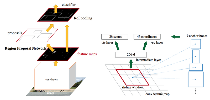
The fundamental idea behind a Faster-RCNN network is that it does two things at once: It detects the bounding boxes of objects of interest using a Region Proposal Network (RPN), and performs classification on those detections using a base classifier after region of interest pooling (ROI).
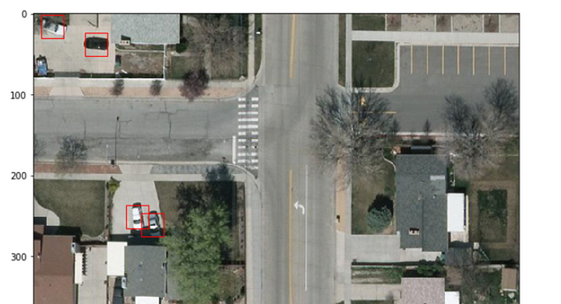
Like our previous attempt, we used COWC for fine-tuning. This time, there is no need to extract individual vehicles for training. To visualize what the dataset looks like, you can test out the following snippet by replacing the (x,y), width and height values in the patches.Rectangle() method with whatever value is shown in an image’s corresponding .txt file.
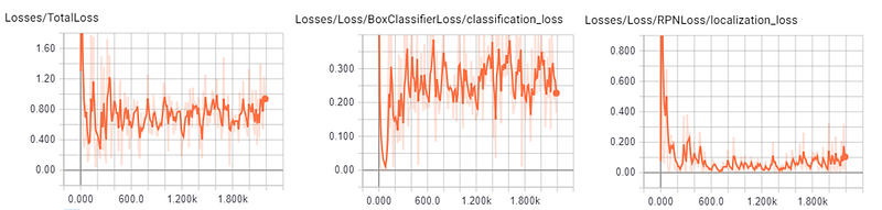
I also had to manually convert these images into Pascal VOC format to be consumed by the Faster R-CNN model. Unlike the classification model, training this model took roughly 24 hours on the K80. This is because in Faster R-CNN, anchor generation within the RPN forms a bottleneck (potentially generating up to 6000 region proposals per image). Other detection models such as SSD or YOLO (at least the first generation) ameliorate the speed issue at the cost of lower mAP scores. However, seeing as we are not concerned with near real-time detection, it suffices to use Faster R-CNN to produce a good output at reasonable speeds (~7 seconds or so on the CPU for each image tile of size of 600x600 which is rescaled from the original 5000x5000 px). Again, Faster R-CNN is provided in the TensorFlow models library. There you can also find some default configuration files for the base classifier you have chosen (ResNet101 pretrained on the MS COCO dataset in my case). There are in fact a whole slew of pretrained base models from TensorFlow’s detection model zoo you can choose for yourself, each with their own speed/mAP trade-off.
This is part of the configuration file I used, note the height and width values that match the COWC “patch_size”, or size of each input image tile. This can be configured in the CreateDetectionScenes.py script from COWC’s Github page. Additionally you can choose to base your classification model on something other than ResNet101. Depending on the size of your detection it may also be prudent to adjust the scales of your anchor for faster convergence, although I find it much more effective to re-tile your inputs if each object ends up comprising less than 4% of your input size.
You can of course write your own evaluation script to visualize the trained model. There is in fact a very good template on TensorFlow’s Github page. I made some modifications to the following snippet to also allow you to adjust the detection threshold and the number of boxes to draw which I find very useful in visually understanding the performance of your model early on in the training process:
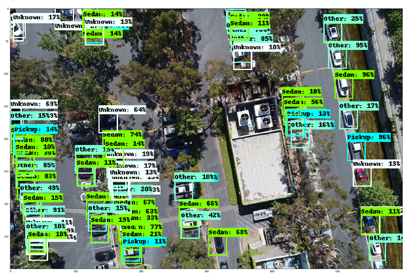
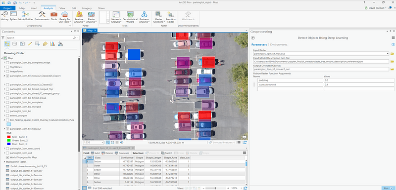
Alternatively, if you wish for a more straightforward approach to performing inferencing, the upcoming ArcGIS Pro 2.3 offers a convenient geoprocessing tool “Detect Objects Using Deep Learning” to perform evaluation on any input raster by passing it a trained model in the form of a frozen inference graph protobuf defined inside a model description JSON file. As well as several evaluation hyperparameters such as padding and detection threshold. Hit run and you get a new feature layer of bounding boxes in return.
Similar to the classification approach, we can visualize these layers much more effectively by exporting them to ArcGIS Online and viewing them in the Operations Dashboard.
All the views from the classification dashboard can also be represented here with the same analyses drawn, but now vehicles parked outside of predesignated spaces (including vehicles in motion) are all detected using Faster R-CNN.
Closing thoughts and future work
This article serves as an exploratory glimpse into machine learning-driven GIS for vehicle detection, and of how important business decisions can be informed from start to finish by leveraging the powerful Esri ecosystem to create a complete BI workflow.
The models described above can of course be taken a couple steps further, by training on an input set with richer annotations or cross-referencing the COWC dataset with datasets that tie together vehicle types with income and other demographic info to produce even more powerful analyses, reveal subtler patterns and yield finer customer segmentations. Likewise, these models apply to aerial detection of all kinds (crops, utility poles, animals, forest fires, ships), as long as you have access to a decent GPU and a fine-tuning dataset.
Another potential expansion to this pipeline would be to introduce oblique imagery into the mix in a manner similar to what was done in Esri’s Oblique Viewer App that allows for multiple oblique views to be attached to the same ortho frame. For vehicle detection this effectively increases the number of images from which we can extract high fidelity data and also gives an unobstructed view of cars hidden under tree canopies.
Hopefully this has been an interesting read, please give us a clap and share this post if you enjoyed it, and let us know in the comments what other insights can be drawn from these data and whether you think there’s a better approach to be considered!
This effort was done as part of the Esri GeoAI team. For other cool GISxML projects, check out the GeoAI Medium page here. Feel free to contact Omar Maherfor internship or full time opportunities! ([email protected])
]]>