How we did it: End-to-end deep learning in ArcGIS
Oil and gas is a huge industry in the United States, and is currently experiencing a boom in the Permian Basin. This oil-rich region stretches from western Texas to eastern New Mexico. Each day, hundreds of new well pads appear across the landscape, making it difficult for regulators to keep up with. But unregistered well pads are both a safety hazard and a missed opportunity for revenue for agencies such as the Bureau of Land Management.
At the plenary session of this year’s Esri Developer Summit, we demonstrated an end-to-end deep learning workflow to find unregistered well pads, using ArcGIS Notebooks. This can help regulators monitor the progress of new drilling on their land as well as look for potential illegal drilling.
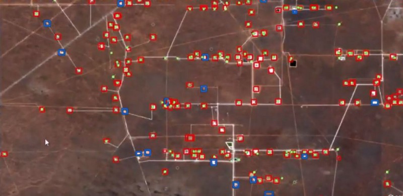
Well Pads detected using deep learning. The ones highlighted in blue are not currently listed in the permits database.
The full workflow, from exporting training data and training a deep learning model to detecting objects across a large landscape, can be done using the ArcGIS API for Python. This blog article, originally written as an ArcGIS Notebook, shows how we did this with the help of the arcgis.learn module.
Geospatial deep learning
The field of artificial intelligence (AI) has progressed rapidly in recent years, matching or in some cases, even surpassing human accuracy. Broadly speaking, AI is the ability of computers to perform a task that typically requires some level of human intelligence. Machine learning is one type of engine that makes this possible, and uses data driven algorithms to learn from data to give you the answers that you need. One type of machine learning that has emerged recently is deep learning. Deep learning refers to deep neural networks, that are inspired from and loosely resemble the human brain.
The arcgis.learn module includes tools that support machine learning and deep learning workflows with geospatial data. This blog post focuses on deep learning with satellite imagery.
Applying Computer Vision to geospatial imagery
One area of AI where deep learning has done exceedingly well is computer vision, i.e. the ability for computers to ‘see’. This is particularly useful for GIS, as satellite, aerial and drone imagery is being produced at a rate that makes it impossible to analyse and derive insight from through traditional means. Object detection and pixel classification are among the most important computer vision tasks and are particularly useful for spatial analysis.
- Object Detection involves finding objects within an image as well as their location in terms of bounding boxes. Finding what is in satellite, aerial or drone imagery, and where, and plotting it on a map can be used for infrastructure mapping, anomaly detection and feature extraction.
- Pixel Classification, also referred to as image segmentation, involves classifying each pixel of an image as belonging to a particular class. In GIS, segmentation can be used for Land Cover Classification or for extracting roads or buildings from satellite imagery.
ArcGIS has tools to help with every step of the deep learning workflow including data preparation and exploratory data analysis, training deep learning models, deploying them for inferencing and finally disseminating results using web layers and maps and driving field activity.
ArcGIS Pro includes tools for labeling features and exporting training data for deep learning workflows and has being enhanced for deploying trained models for feature extraction or classification. ArcGIS Image Server in the ArcGIS Enterprise 10.7 release has similar capabilities and allow deploying deep learning models at scale by leveraging distributed computing. ArcGIS Notebooks provide one-click access to pre-configured Jupyter Notebooks along with the necessary deep learning libraries and a gallery of starter notebooks that show how deep learning models can be easily trained and deployed.
The arcgis.learn module
The arcgis.learn module in ArcGIS API for Python enable GIS analysts and data scientists to easily adopt and apply deep learning in their workflows. It enables training state-of-the-art deep learning models with a simple, intuitive API. By adopting the latest research in deep learning, it allows for much faster training and removes guesswork in the deep learning process. It integrates seamlessly with the ArcGIS platform by consuming the exported training samples directly, and the models that it creates can be used directly for inferencing (object detection and pixel classification) in ArcGIS Pro and Image Server.
This module includes methods and classes for:
- Exporting Training Data
- Data Preparation
- Model Training
- Model Management
- Inference
Prerequisites
Data preparation, augmentation and model training workflows using arcgis.learn have a dependency on PyTorch and fast.ai deep learning libraries.
If you are using ArcGIS Notebook Server, the dependencies are already installed.
In the ArcGIS Pro 2.3 Python environment, the dependencies need to be installed using these commands:
conda install -c conda-forge spacy
conda install -c pytorch pytorch=1.0.0 torchvision
conda install -c fastai fastai=1.0.39
conda install -c arcgis arcgis=1.6.0 --no-pin
Otherwise, in a new conda environment, issue the following commands:
conda install -c fastai -c pytorch -c esri fastai=1.0.39 pytorch=1.0.0 torchvision arcgis=1.6.0
Object Detection with arcgis.learn
Deep learning models ‘learn’ by looking at several examples of imagery and the expected outputs. In the case of object detection, this requires imagery as well as known (or labelled) locations of objects that the model can learn from. With the ArcGIS platform, these datasets are represented as layers, and are available in our GIS.
In the workflow below, we will be training a model to identify well pads from Sentinel-2 imagery. Sentinel-2 is an Earth observation mission developed by ESA as part of the Copernicus Programme to perform terrestrial observations in support of services such as forest monitoring, land cover change detection, and natural disaster management.
In this analysis, data downloaded from https://earthexplorer.usgs.gov/ has been used for creating hosted image service in our GIS. The code below connects to our GIS and accesses the known well pad locations and the Sentinel imagery:
from arcgis.gis import GIS
from arcgis.raster.functions import apply
from arcgis.learn import export_training_data
gis = GIS("home")
# layers we need - The input to generate training samples and the imagery
well_pads = gis.content.get('ae6f1c62027c42b8a88c4cf5deb86bbf') # Well pads layer
well_pads
# Sentinel-2 imagery published to portal
sentinel_item = gis.content.get("15c1069f84eb40ff90940c0299f31abc")
sentinel_item
Exporting Training Samples
The export_training_data() method generates training samples for training deep learning models, given the input imagery, along with labeled vector data or classified images. Deep learning training samples are small subimages, called image chips, and contain the feature or class of interest. This tool creates folders containing image chips for training the model, labels and metadata files and stores them in the raster store of your enterprise GIS. The image chips are often small, such as 256 pixel rows by 256 pixel columns, unless the training sample size is larger. These training samples support model training workflows using the arcgis.learn package as well as by third-party deep learning libraries, such as TensorFlow or PyTorch.
The object detection models in arcgis.learn accept training samples in the PASCAL_VOC_rectangles (Pattern Analysis, Statistical Modeling and Computational Learning, Visual Object Classes) format. The PASCAL VOC dataset is a standardized image dataset for object class recognition. The label files are XML files and contain information about image name, class value, and bounding boxes.
The models in arcgis.learn take advantage of pretrained models, that have been trained on large image collections, such as ImageNet, and fine tune them on satellite imagery. Pretrained models like these are excellent feature extractors and can be fine-tuned relatively easily on another task or different imagery without needing as much data. However, since the photographs that these models have been trained on contain only 3 channels (Red, Green Blue), we cannot take advantage of all the bands available in multispectral imagery, and need to pick 3.
The extract_bands() method can be used to specify which 3 bands should be extracted for fine tuning the models. In our analysis, we will be using the pre-configured ‘Natural Color with Dynamic Rage Adjustment(DRA)’ raster function:
sentinel_data = apply(sentinel_item.layers[0], 'Natural Color with DRA', astype='U8')
For better training, image chips should be exported with a larger size than that used for training the models. This allowsarcgis.learn to perform random center cropping as part of it's default data augmentation and makes the model see a different sub-area of each chip when training leading to better generalization and avoid overfitting to the training data. By default, a chip size of 448 x 448 pixels works well, but this can be adjusted based on the amount of context you wish to provide to the model, as well as the amount of GPU memory available.
Here, we are exporting the training data for our model in the well_pads folder:
export_training_data(sentinel_data, well_pads, "PNG",
{"x":448,"y":448}, {"x":224,"y":224},
"PASCAL_VOC_rectangles", 75,
"well_pads")
Data Preparation
Once the training samples have been exported, they need to be fed into the model for training. Data preparation can be a time consuming process that involves collating and massaging the training chips and labels into the specific format needed by each deep learning model.
Typical data processing piplelines involve splitting the data into training and validation sets, applying various data augmentation techniques, creating the necessary data structures for loading data into the model, setting the appropriate batch size and so on.arcgis.learn automates all these time consuming tasks and the prepare_data() method can directly read the training samples exported by ArcGIS. The prepare_data() method inspects the format of the training samples exported by export_training_data tool in ArcGIS Pro or Image Server (whether for object detection or pixel classification) and constructs the appropriate fast.aiDataBunch from it. This DataBunch consists of training and validation DataLoaders with the specified transformations for data augmentations, chip size, batch size, and split percentage for train-validation split.
By default, prepare_data uses a default set of transforms for data augmentation, that work well for satellite imagery. These transforms randomly rotate, scale and flip the images so the model sees a different image each time. This helps the model generalize better and not just ‘remember’ or overfit to the specific images in the training set. Alternatively, users can compose their own transforms usingfast.ai transforms for the specific data augmentations they wish to perform.
from arcgis.learn import prepare_data
data = prepare_data('/arcgis/directories/rasterstore/well_pads',
{0: ' Pad'})
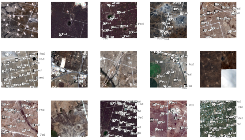
The show_batch() method can be used to visualize the exported training samples, along with labels, after data augmentation transformations have been applied.
data.show_batch()
Model Training
arcgis.learn includes support for training deep learning models for object detection. Support for training pixel classification model is coming in the next release.
The models in arcgis.learn are based upon pretrained Convolutional Neural Networks (CNNs, or in short, convnets) that have been trained on millions of common images such as those in the ImageNet dataset for image classification tasks. These CNNs (such as Resnet, VGG, Inception, etc.) can classify what’s in an image by basing their decision on features that they learn to identify in those images. In particular, they use a hierarchy of layers, with the earlier layers learning to identify simple features like edges and blobs, middle layers combining these primitive features to identify corners and object parts and the later layers combining the inputs from these in unique ways to grasp what the whole image is about (i.e. the semantic meaning). The final layer in a typical convnet is a ‘fully connected’ layer that looks at all the extracted semantic meaning in the form of feature maps across the whole image and essentially does a weighted sum of these to come up with a probability of each object class (whether its an image of a cat or a dog, or whatever).
A convnet trained on a huge corpus of images such as ImageNet is thus considered as a ready-to-use feature extractor. We could replace the last few layers of these convnets and substitute it with something else that uses those features for other useful tasks, such as object detection and pixel classification.
The arcgis.learn module is based on PyTorch and fast.ai and enables fine-tuning of pretrained torchvision models on satellite imagery. Pretrained models like these are excellent feature extractors and can be fine-tuned relatively easily on another task or different imagery without needing as much data. The arcgis.learn models leverages fast.ai's learning rate finder and one-cycle learning, and allows for much faster training and removes guesswork in the deep learning process.
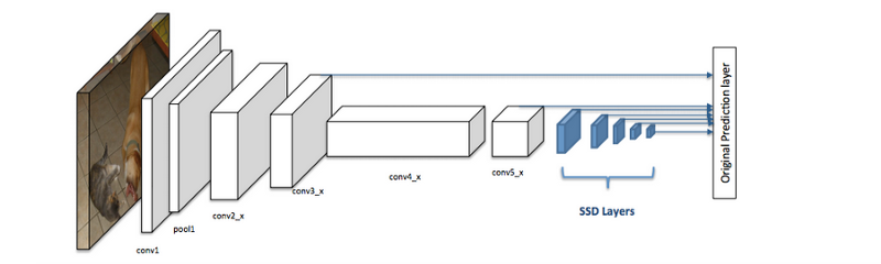
arcgis.learn includes the SingleShotDetector model (based on Fast.ai MOOC Version2 Lesson 9) for object detection tasks. A pretrained convnet, like ResNet, acts as the 'backbone' upon which the SingleShotDetectormodel is based, or as the 'encoder' part of the upcomingUnetClassifier.
Object Detection using SingleShotDetector
Once we have a good image classifier, a simple way to detect objects is to slide a ‘window’ across the image and classify whether the image in that window (cropped out region of the image) is of the desired type. However, this is terribly inefficient as we need to look for objects everywhere in the image, and at different scales, as the objects might be larger or smaller. This requires multiple passes of regions of the image through the image classifier which is computationally infeasible. Another class of object detection networks (like R-CNN and Fast(er) R-CNN) use a two stage approach — first to identify regions where objects are expected to be found and then running those region proposals through the convnet for classifying and creating bounding boxes around them.
The latest generation of object detection networks such as YOLO (You Only Look Once) and SSD (Single-Shot Detector) use a fully convolutional approach in which the network is able to find all objects within an image in one pass (hence ‘single-shot’ or ‘look once’) through the convnet.
“SSD: Single Shot MultiBox Detector”, 2015; arXiv:1512.02325.
Instead of using a region proposal networks to come up with candidate locations of prospective objects, the Single Shot MultiBox Detector (on which the SingleShotDetector is modeled) divides up the image using a grid with each grid cell responsible for predicting which object (if any) lies in it and where.
Backbone SSD uses a pre-trained image classification network as a feature extractor. This is typically a network like ResNet trained on ImageNet, from which the final fully connected layers to come up with the predicted class of an input image have been removed. We are thus left with a deep neural network that is able to extract semantic meaning from the input image while preserving the spatial structure of the image albeit at a lower resolution. For ResNet34 the backbone results in a 256 7x7 ‘feature maps’ of activations for each input image. Each of these 256 feature maps can be interpreted as a grid of 7x7 activations that fire up when a particular feature is detected in the image. In the SSD architecture, one or more convolutional layers are added to this backbone and the outputs are interpreted as the bounding boxes and classes of objects in the spatial location of the final layer’s activations.
Receptive Field Convolutional neural networks preserve the spatial structure of an image because of the way the convolution operation is applied. A learnable filter slides over the image from left to right and top to bottom and the activations represent how similar that part of the image is to the filter. Each activation in the output feature map is thus ‘looking at’ that region of the previous feature map (and ultimately the image because a deep CNN has multiple such convolutional layers). The part of the image that is ultimately responsible for an activation in a feature map is referred to as the ‘receptive field’ of that activation. Each activation in the output feature map has ‘seen’ that part of the image more than any other activation and is it natural to expect that activation to contain the most information needed to detect objects in its receptive field. This is the central premise of the SSD architecture.
As it’s possible for multiple objects to occupy a grid cell, and for the objects to have a different sizes or aspect ratios, each grid cell has several assigned anchor boxes (also known as prior boxes) — one for each possible object size and aspect ratio within that grid cell. SSD uses a matching phase while training, to match the appropriate anchor box with the bounding boxes of each ground truth object within an image. Essentially, the anchor box with the highest degree of overlap with an object is responsible for predicting that object’s class and its location. This property is used for training the network and for predicting the detected objects and their locations once the network has been trained.
Having a knowledge of the SingleShotDetector architecture and how the anchor boxes are specified using grid cells, aspect ratios and zoom levels allows one to design a suitable model for the object detection task at hand. If the objects you are detecting are all of roughly the same size, you can simplify the network architecture by using just one scale of the anchor boxes. A simpler network is easier to train. More powerful networks can detect multiple overlapping objects of varying sizes and aspect ratios, but need more data and computation for training.
Grid cells A simple way to detect multiple objects in an image is to divide the image using a grid and have each grid cell be responsible for detecting objects in that region of the image. Detecting objects simply means predicting the class(type) and location of an object within that region. If no object is present, we consider it as the background class and the location is ignored.
In the SSD architecture, we add additional convolutional layers to the backbone network and architect the additional layers in such a manner that the spatial size of the final layer is the same as the size of the grid we are using. The depth of the final feature map is used to predict the class of the object within the grid cell and it’s bounding box. This allows SSD to be a fully convolutional network that is fast and efficient, while taking advantage of the receptive field of each grid cell to detect objects within that grid cell.
For instance, we could use a 4x4 grid to detect objects in an image, when we see that their size is such that approximately 16 of them could occupy an image chip (4 on a side).
Such an SSD architecture can be created using:
ssd = SingleShotDetector(data, grids=[4], zooms=[1.0], ratios=[[1.0, 1.0]])
The grids parameter specifies the size of the grid cell, in this case 4x4. Additionally, we are specifying a zoom level of 1.0 and aspect ratio of 1.0:1.0. What this essentially means is that the network will create an anchor box (or prior box, as its known in other places) for each grid cell, which is the same size as the grid cell (zoom level of 1.0) and is square in shape with an aspect ratio of 1.0:1.0 The output activations along the depth of the final feature map are used to shift and scale this anchor box (within a reasonable limit) so it can approach the actual bounding box of the object even if it doesn’t exactly line up with the anchor box.
We might be interested in several layers or hierarchies of grid cells. For example, we could use a 4x4 grid to find smaller objects, a 2x2 grid to find mid sized objects and a 1x1 grid to find objects that cover the entire image. That can be done by specifying [4, 2, 1] as the grids parameter.
Zoom levels/scales
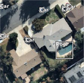
Cars and Pools have different scales
It is not necessary for the anchor boxes to have the same size as the grid cell. We might be interested in finding smaller or larger objects within a grid cell. The zooms parameter is used to specify how much the anchor boxes need to be scaled up or down with respect to each grid cell.
Aspect ratios
Not all objects are square in shape. Some are longer and some are wider, by varying degrees. The SSD architecture allows pre-defined aspect ratios of the anchor boxes to account for this. The ratios parameter can be used to specify the different aspect ratios of the anchor boxes associates with each grid cell at each zoom/scale level.
Having multiple anchor boxes per grid cell with different aspect ratios and at different scales, while also allowing for multiple hierarchies of grid cells results in a profusion of potential anchor boxes that are candidates for matching the ground truth while training, and for prediction.
Creating SingleShotDetector Model
Since the image chips visualized in the section above indicate that most well pads are roughly of the same size and square in shape, we can keep an aspect ratio of 1:1 and zoom (scale) of 1. This will help simplify the model and make it easier to train. Also, since the size of well pads in the image chips is such that approximately nine could fit side by side, we can keep a grid size of 9.
We then create a Single Shot Detector with a specified grid size, zoom scale and aspect ratio:
from arcgis.learn import SingleShotDetector
ssd = SingleShotDetector(data, grids=[9], zooms=[1.0], ratios=[[1.0, 1.0]])
Finding the optimum learning rate
Once the appropriate model has been constructed, it needs to be trained over several epochs, or training passes over the training data. This process involves setting the optimum learning rate. Picking a very small learning rate leads to slow training of the model, while picking one that it too high can prevent the model from converging and ‘overshoot’ the minima, where the loss (or error rate) is lowest. arcgis.learn includes fast.ai's learning rate finder, accessible through the model's lr_find() method, that helps in picking the optimum learning rate, without needing to experiment with several learning rates and picking from among them.
ssd.lr_find()
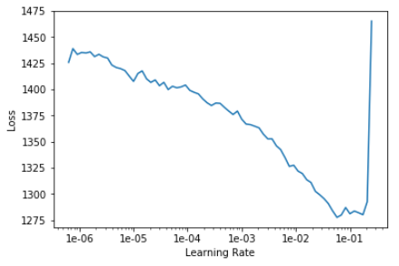
The learning rate is specified using two numbers - a lower rate for fine tuning the earlier layers of the pretrained backbone, and the higher rate for training the newly added layers for the task at hand. The higher learning rate can be deduced by inspecting the learning rate graph and picking the highest learning rate (on the x axis) where the loss is still going down (while still being lower than the point from where it shoots up). The lower learning rate is usually a fraction (one tenth works well) of the higher rate but can be adjusted depending upon how different the imagery is from natural images on which the backbone network is trained.
In the chart above we find that the loss is going down steeply at 2e-02 (0.02) and we pick that as the higher learning rate. The lower learning rate is approximately one tenth of that. We choose 0.001 to be more careful not to disturb the weights of the pretrained backbone by too much. This is why we are picking a learning rate of slice(0.001, 0.02) to train the model in the next section.
Training the model
Training the model is an iterative process. We can train the model using its fit() method till the validation loss (or error rate) continues to go down with each epoch (or training pass over the data). This is indicative of the model learning the task.
ssd.fit(10, slice(0.001, 0.02))

As each epoch progresses, the loss (error rate, that we are trying to minimize) for the training data and the validation set are reported. In the table above we can see the losses going down for both the training and validation datasets, indicating that the model is learning to recognize the well pads. We continue training the model for several iterations like this till we observe the validation loss starting to go up. That indicates that the model is starting to overfit to the training data, and is not generalizing well enough for the validation data. When that happens, we can try reducing the learning rate, adding more data (or data augmentations), increase regularization by increasing the dropoutparameter in the SingleShotDetector model, or reduce the model complexity.
Unfreezing the backbone and fine-tuning
By default, the earlier layers of the model (i.e. the backbone or encoder) are frozen and their weights are not updated when the model is being trained. This allows the model to take advantage of the (ImageNet) pretrained weights for the backbone, and only the ‘head’ of the network is trained initially. Once the later layers have been sufficiently trained, it helps to improve model performance and accuracy to unfreeze() the earlier layers and allow their weights to be fine-tuned to the nuances of the particular satellite imagery compared to the photos of everyday objects (from ImageNet) that the backbone was trained on. The learning rate finder can be used to identify the optimum learning rate between the different training phases .
Visualizing results
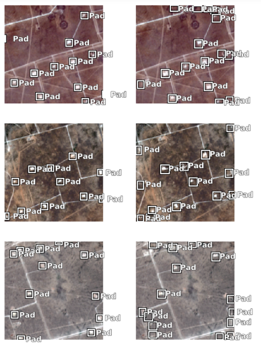
The results of how well the model has learnt can be visually observed using the model’s show_results() method. The ground truth is shown in the left column and the corresponding predictions from the model on the right. As we can see below, the model has learnt to detect well pads fairly well. In some cases, it is even able to detect the well pads that are missing in the ground truth data (due to inaccuracies in labeling or the records).
ssd.show_results(rows=25, thresh=0.05)
Saving trained model
Once you are satisfied with the model, you can save it using the save()method. This creates an Esri Model Definition (EMD file) that can be used for inferencing in ArcGIS Pro as well as a Deep Learning Package (DLPK zip) that can be deployed to ArcGIS Enterprise for distributed inferencing across a large geographical area. Saved models can also be loaded back using the load()method, for futher fine tuning.
ssd.save('WellPadDetector')
> Created model files at /arcgis/directories/rasterstore/well_pads/models/WellPadDetector
Deploying model
Once a model has been trained, it can be added to ArcGIS Enterprise as a deep learning package.
trained_model = '/arcgis/directories/rasterstore/well_pads/models/WellPadDetector/WellPadDetector.zip'
model_package = gis.content.add(item_properties={
"type":"Deep Learning Package",
"typeKeywords":"Deep Learning, Raster",
"title":"Well Pad Detection Model",
"tags":"deeplearning",
"overwrite":'True'}, data=trained_model)
model_package
Model lifecycle management
The arcgis.learn module includes the install_model() method to install the uploaded model package (*.dlpk) to the raster analytics server.
Optionally after inferencing the necessary information from the imagery using the model, the model can be uninstalled usinguninstall_model(). The deployed models on an Image Server can be queried using the list_models()method.
The uploaded model package is installed automatically on first use as well. We can query the settings of the deep learning model using the query_info().
from arcgis.learn import Model
detect_objects_model = Model(model_package)
detect_objects_model.install()
Detecting Objects
The detect_objects() function can be used to generate feature layers that contains bounding box around the detected objects in the imagery data using the specified deep learning model.
Note that the deep learning library dependencies needs to be installed separately, in addition on the image server.
For arcgis.learn models, the following sequence of commands in ArcGIS Image Server’s Pro Python environment install the necessary dependencies:
conda install -c conda-forge spacy
conda install -c pytorch pytorch=1.0.0 torchvision
conda install -c fastai fastai=1.0.39
conda install -c arcgis arcgis=1.6.0 --no-pin
We specify the geographical extent and imagery cell size for feature extraction, and whether to use the GPU or CPU in the contextparameter. Each detection has an associated score, that indicates how confident the model is about that prediction. We can set a score threshold to filter out false detections. In this case, we found that we can lower the score threshold to 0.05 and catch more detections without having too many false detections. A non max suppression(nms_overlap) parameter can be specified to weed out duplicate overlapping detections of the same object.
context = {'cellSize': 10,
'processorType':'GPU',
'extent':{'xmin': -11587791.393960,
'ymin': 3767970.198031,
'xmax': -11454320.817016,
'ymax': 3875304.476397, 'spatialReference': {'latestWkid': 3857, 'wkid': 102100}}}
params = {'padding':'0', 'threshold':'0.05', 'nms_overlap':'0.1', 'batch_size':'64'}
Finally, the code below shows how we can use distributed raster analytics to automate object detection across a large geographical area and create a feature layer of well pad detections.
from arcgis.learn import detect_objects
detected_pads = detect_objects(input_raster=sentinel_data,
model=detect_objects_model,
model_arguments=params,
output_name="Well_Pads_Detect_full3",
context=context,
gis=gis)
detected_pads
Visualizing detection layer
We can visualize the results using the map widget, right within the notebook.
web_map = gis.content.search("title: Well Pad Detection AND owner:portaladmin",item_type="Web Map")[0]
map_widget = gis.map(web_map)
map_widget.extent = {'spatialReference': {'latestWkid': 3857, 'wkid': 102100},
'xmin': -11397184.938845266,
'ymin': 3761693.7641860787,
'xmax': -11388891.521276105,
'ymax': 3764082.4213200537}
map_widget.zoom = 15
map_widget
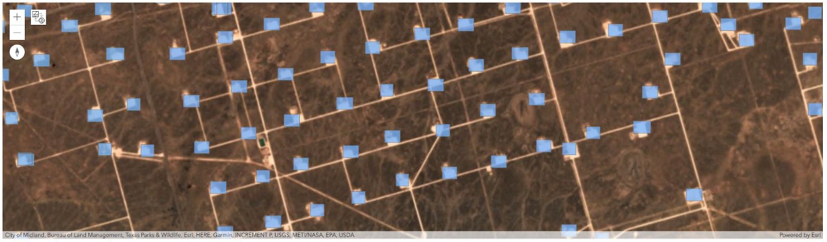
We could take these results, share them as maps and layers, do further analysis to find which well pads are missing in the database, where the hotspots of new drilling activity are, and how they are changing over time. With Workforce for ArcGIS, we can create assignments for mobile workers, such as inspectors and drive field activity. In conclusion, ArcGIS has end-to-end support for deep learning — from hosting the data, to exporting training samples and training a deep learning model, to detecting objects across a large region and driving field activity.